A blog post by Christian Robert considered an ancient (2011!) article titled "Bayesian assessment of null values via parameter estimation and model comparison." Here I'll try to clarify the ideas from way back then through the lens of more recent diagrams from my workshops and a new article.
Terminology: "Bayesian assessment of null values" is supposed to be neutral wording to refer to any Bayesian method for assessing null values. Bayesian "hypothesis testing" is reserved for Bayes factors. Making decisions by posterior interval is not referred to as hypothesis testing and is not equivalent to Bayes factors.
Bayesian hypothesis testing: Suppose we are modeling some data with a model that has parameter δ in which we are currently interested, along with some other parameters. A null hypothesis model can be formulated as a prior on the parameters that puts a "spike" at the null value of δ but is spread out over the other parameters. A non-null alternative model puts a prior on δ that allows non-null values. The two models are indexed by a higher-level discrete parameter M. The entire hierarchy (a mixture model) has all its parameters updated by the data. The following slide from my workshops illustrates:
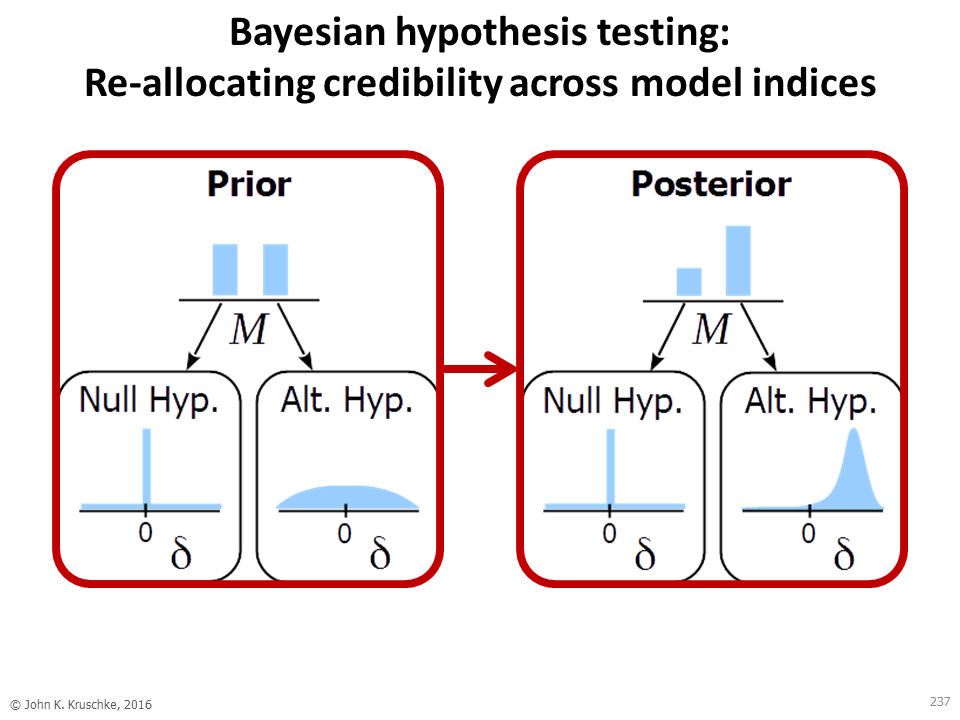
The Bayes factor (BF) is the shift in model-index probabilities:


Digression: I throw in two usual caveats about using Bayes factors. First, Bayesian model comparison --for null hypothesis testing or more generally for any (non-nested) models-- must use meaningful priors on the parameters in both models for the Bayes factor to be meaningful. Default priors for either model are typically not very meaningful and quite possibly misleading.

 |
| Link in slide above: http://doingbayesiandataanalysis.blogspot.com/2015/12/lessons-from-bayesian-disease-diagnosis_27.html |
Assessing null value through parameter estimation: There's another way to assess null values. This other way focuses on the (marginal) posterior distribution of the parameter in which we're interested. (As mentioned at the outset, this approach is not called "hypothesis testing.") This approach is analogous to frequentist equivalence testing, which sets up a region of practical equivalence (ROPE) around the null value of the parameter:

The logic of this approach stems from a direct reading of the meaning of the intervals. We decide to reject the null value when the 95% highest density parameter values are all not practically equivalent to the null value. We decide to accept the null value when the 95% highest density parameter values are all practically equivalent to the null value. Furthermore, we can make direct probability statements about the probability mass inside the ROPE such as, "the probability that the parameter is practically equivalent to the null is 0.017" or "the probability that the parameter is practically equivalent to the null is 0.984."
The ROPE is part of the decision rule, not part of the null hypothesis. The ROPE does not constitute an interval null hypothesis; the null hypothesis here is a point value. The ROPE is part of the decision rule for two main purposes: First, it allows decisions to accept the null (again, analogous to frequentist equivalence testing). Second, it makes the decision rule asymptotically correct: As data sample size increases, the rule will come to the correct decision, either practically equivalent to the null value (within the ROPE) or not (outside the ROPE).
Juxtaposing the two approaches: Notice that the two approaches to assessing null values are not equivalent and have different emphases. The BF focuses on the model index, whereas the HDI and ROPE focus on the parameter estimate:

Below is an example of the different information provided by hypothesis testing and estimation (for both frequentist and Bayesian analyses). The data are dichotomous, with z=14 successes out N=18 attempts (e.g., 14 heads out of 18 flips). The data are modeled by a Bernoulli distribution with parameter θ. The null value is taken to be θ=0.50. For the Bayesian analysis, the alternative-hypothesis prior is uniform merely for purposes of illustration; uniform is equivalent to dbeta(1,1).
You can see above that Bayesian hypothesis testing and Bayesian parameter estimation provide very different information. Which approach to use for assessing the null value then comes down to careful interpretation and practicalities. For more discussion please see this article: Kruschke, J. K. and Liddell, T. (2017), The Bayesian New Statistics: Hypothesis testing, estimation, meta-analysis, and power analysis from a Bayesian perspective. Psychonomic Bulletin & Review.

A comparison of frequentist equivalence testing with HDI+ROPE appears in a subsequent blog post: http://doingbayesiandataanalysis.blogspot.com/2017/02/equivalence-testing-two-one-sided-test.html
ReplyDelete